The Transformer Revolution
Master the transformer architecture that powers modern AI - understand self-attention, multi-head attention, and why this architecture changed everything
Section 1: Attention Is All You Need
The AI Timeline Before 2017
In 2017, deep learning was already successful but hitting walls. Convolutional Neural Networks dominated computer vision. They were great at images but struggled with sequences like text, speech, and time series data.
Recurrent Neural Networks and their variants like LSTMs and GRUs handled sequences. They could process text word by word, maintaining a hidden state that captured context. But they had fatal flaws.
The sequential bottleneck meant each word had to be processed before the next. No parallelization meant slow training. Vanishing gradients caused information from early in a sequence to degrade over time. Long-range dependencies were hard to learn. The fixed capacity of hidden states meant they had to compress all context into a fixed-size vector. More context meant more compression loss.
Machine translation exemplified these struggles. State-of-the-art systems used sequence-to-sequence models where an RNN encoder processed the source sentence into a context vector, then an RNN decoder generated the translation. They worked, but poorly for long sentences and slowly for everything.
The Paper That Changed Everything
In June 2017, a team at Google Brain and Google Research published “Attention Is All You Need.” The title was a provocation. The prevailing wisdom was that attention mechanisms were useful additions to RNNs. This paper claimed you could throw out the RNN entirely and build everything from attention.
The results were striking. Better quality meant state-of-the-art translation on WMT 2014 English-to-German with BLEU score 28.4, improving by more than 2 points. Faster training meant training time reduced from 3.5 days to 12 hours on the same hardware. Simpler design meant the architecture was more elegant, more parallelizable, and more interpretable.
Within months, transformers started dominating NLP. Within two years, BERT in 2018 and GPT-2 in 2019 showed that pre-trained transformers could be fine-tuned for almost any language task. By 2020, GPT-3 demonstrated few-shot learning at scale. By 2022, ChatGPT brought transformers to mainstream awareness.
A neural network architecture based entirely on attention mechanisms, introduced in the 2017 paper “Attention Is All You Need.” Transformers process sequences by letting every position directly attend to every other position, solving the parallelization and long-range dependency problems that limited RNNs. This architecture underlies all modern large language models.
What Problem Did Transformers Solve?
The core insight is that all inputs should be able to attend to all other inputs simultaneously.
In RNNs, information flows sequentially. Word 1 affects word 2, which affects word 3, and so on. To connect word 1 to word 50, information must traverse 49 steps, degrading along the way.
In transformers, word 1 can attend directly to word 50. Every position can look at every other position in one step. This enables parallelization where all positions process simultaneously and training becomes massively parallelizable on GPUs. It enables long-range dependencies where direct connections mean no degradation over distance. It enables dynamic weighting where the model learns which connections matter, rather than treating all sequential connections equally.
The fundamental mechanism enabling this is self-attention. Let us understand how it works.
Section 2: Self-Attention Mechanism
The Intuition: Dynamic Relevance
Imagine reading this sentence: “The animal didn’t cross the street because it was too tired.”
What does “it” refer to? Your brain instantly resolves this. “It” means the animal, not the street. You do this by paying attention to context. “Tired” relates to animals, not streets.
Self-attention formalizes this intuition. For each word, the mechanism looks at all other words in the sequence, computes how relevant each word is to the current word, and creates a new representation that mixes information based on relevance.
Consider a simpler example: “The cat sat on the mat.”
For the word “cat”, self-attention might determine that “The” has low relevance as it is just an article, “cat” itself has high relevance for self-reference helping with identity, “sat” has high relevance as this is what the cat did, “on” has medium relevance as a preposition indicating relationship, “the” has low relevance, and “mat” has medium relevance as the location of sitting.
The output representation of “cat” would be a weighted combination of all these words, with “cat” and “sat” contributing most.
The Math: Query, Key, Value
Self-attention implements this through three learned transformations of each input.
Query represents “What am I looking for?” Key represents “What information do I contain?” Value represents “What information should I pass along?”
The Database Analogy
Think of Query, Key, and Value like a database lookup system. Query is your search term. Key is the index you search against. Value is the actual data you retrieve. The dot product between Query and Key determines relevance, and that relevance weights how much of each Value contributes to the output.
For each position in the sequence, first transform inputs by applying learned weight matrices to create Q, K, V vectors. Q equals X times W_Q, K equals X times W_K, and V equals X times W_V.
Next compute attention scores. For each position, compute how much it should attend to every position. The score from position i to j equals Q_i dot K_j. This measures compatibility: how well position i’s query matches position j’s key.
Then normalize with softmax to convert scores to probabilities that sum to 1. Attention from i to j equals softmax of the score, dividing by the square root of d_k for stable gradients.
Finally create a weighted combination by mixing values according to attention weights. Output_i equals the sum over j of Attention times V_j.
The Equation
The complete self-attention equation, as written in the original paper:
Attention(Q, K, V) = softmax(QK^T / sqrt(d_k)) VQK transposed is matrix multiplication of queries with keys transposed. This computes all pairwise compatibility scores at once. Dividing by the square root of d_k scales by the square root of key dimension. This prevents dot products from becoming too large, which would push softmax into saturation regions with tiny gradients. Softmax converts each row of scores to probabilities where each row sums to 1. Multiplying by V computes the weighted combinations.
The genius is that everything happens in parallel. All positions compute their attention simultaneously. A single matrix multiplication computes all pairwise interactions.
Concrete Example with Numbers
Let us trace through a tiny example with the sequence “cat sat” embedded as 4-dimensional vectors.
Starting with input embeddings, “cat” is represented as [1.0, 0.5, 0.3, 0.8] and “sat” as [0.2, 0.9, 0.7, 0.1].
With learned weight matrices that project to 2D for simplicity, we create Q, K, V vectors for each token. Then we compute attention scores using dot products, scale and apply softmax to get attention weights, and finally compute the weighted sum of values.
Through this process, the output representation of “cat” now incorporates information from both “cat” and “sat”, weighted by their relevance. If the attention weight from “cat” to itself is 0.52 and to “sat” is 0.48, then the output mixes roughly half of each token’s value vector.
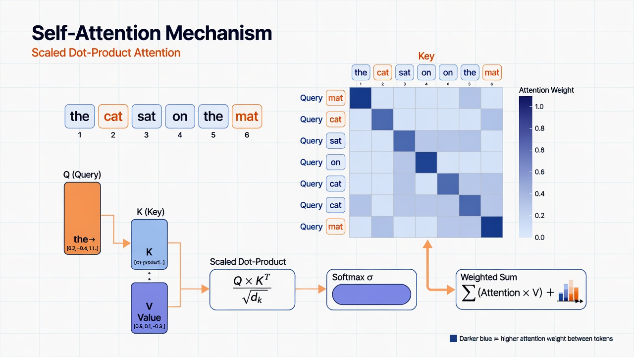
This diagram illustrates how self-attention computes dynamic, content-based relevance scores across all pairs of tokens in parallel.
Why Self-Attention Works
Self-attention succeeds because relevance is learned, not fixed. The Q, K, V transformations are learned parameters. The model discovers what makes words relevant to each other through training. This content-based addressing means “cat” can attend strongly to “sat” or weakly to it based on learned semantics, not just position.
What Self-Attention Cannot Do (Yet)
Self-attention has no inherent sense of position. “Cat sat mat” and “mat sat cat” produce the same attention patterns without positional information. We address this with positional encoding later.
Self-attention is also O(n squared) in sequence length: every position attends to every position. For a 1000-word document, that is 1,000,000 interactions. This becomes the bottleneck for very long sequences.
Section 3: Multi-Head Attention
Why Multiple Attention Heads?
Self-attention lets the model learn one pattern of relevance. But language has many types of relationships.
Syntactic relationships include subject-verb agreement and pronoun resolution. Semantic relationships include thematic similarity, contradiction, and entailment. Positional relationships capture nearby words and distant dependencies. Functional relationships connect modifiers to nouns and arguments to verbs.
A single attention mechanism must compromise between these. Multi-head attention runs several attention mechanisms in parallel, each learning different patterns.
The Architecture
Instead of one set of Q, K, V transformations, use h parallel heads (typically h equals 8 or 16). For each head i, create separate Q_i, K_i, V_i by projecting inputs through different weight matrices. Compute attention separately for each head. Concatenate all head outputs and apply a final linear transformation.
MultiHead(Q,K,V) = Concat(head_1, ..., head_h) × W_O

where head_i = Attention(QW^Q_i, KW^K_i, VW^V_i)
Each head has its own learned weight matrices. Each learns its own attention patterns. The outputs are concatenated and linearly transformed.
Intuitive Example
Consider the sentence: “The bank can guarantee deposits will eventually cover future tuition costs because it has reliable income.”
Different heads might specialize in different ways.
Head 1 focused on syntactic patterns might connect “bank” to “can” for subject-verb agreement, “it” to “bank” for pronoun resolution, and “deposits” to “cover” for another subject-verb relationship.
Head 2 focused on financial semantics might connect “bank” strongly to “deposits”, “guarantee”, and “income” while connecting “costs” to “tuition” and “cover”.
Head 3 focused on temporal semantics might connect “eventually” to “future” and “will” while connecting “costs” to “future”.
Head 4 focused on causal reasoning might connect “guarantee” to “because” and “because” to “has” and “income”.
Each head forms a different understanding of the sentence. The model learns to route different aspects of meaning through different heads.
Running multiple attention mechanisms in parallel, each with separate learned Q, K, V transformations. Different heads learn to capture different types of relationships (syntactic, semantic, positional). Outputs are concatenated and combined, providing multiple perspectives on the input data.
Empirical Observations
Researchers have analyzed what different heads learn in trained models.
Positional heads attend primarily to adjacent words or words at fixed relative positions. These capture local n-gram patterns.
Syntactic heads learn to follow syntactic dependencies connecting subjects to verbs, adjectives to nouns, and pronouns to antecedents.
Semantic heads group semantically related words, connecting “bank” with financial terms when used in financial contexts.
Rare heads develop specialized, hard-to-interpret patterns that nonetheless improve performance.
Importantly, this specialization emerges from training. Heads are not designed for specific roles. They learn them.
Section 4: The Complete Transformer Block
Beyond Attention: The Full Architecture
Self-attention is the star, but a complete transformer block includes several other crucial components. Each serves a specific purpose in making the model trainable and effective.
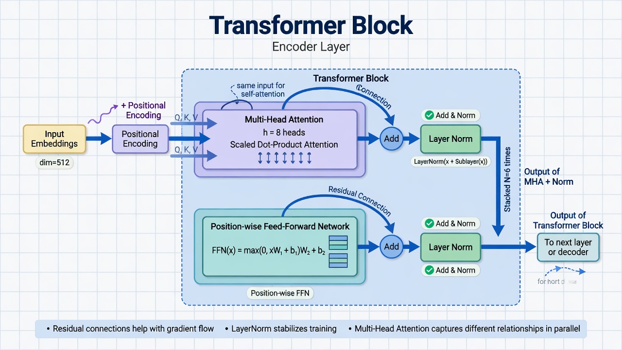
A single transformer layer (block) combines attention, feed-forward processing, residuals, and normalization. Dozens or hundreds of these are stacked.
A single transformer block consists of multi-head self-attention, add and normalize operations with residual connections and layer normalization, a position-wise feed-forward network, and another add and normalize operation.
Residual Connections
Deep networks face the vanishing gradient problem. As gradients backpropagate through many layers, they can become vanishingly small, making learning slow or impossible.
Residual connections from ResNet in 2015 solve this. Instead of learning output equals F(input), the layer learns the residual: output minus input equals F(input), so output equals F(input) plus input.
This creates gradient highways. Gradients can flow backward through the identity connection without being diminished by transformations. Even if F contributes little, the gradient passes through.
In transformers, after attention, x becomes x plus MultiHeadAttention(x). After feed-forward, x becomes x plus FeedForward(x). The input is always added back. If attention or the feed-forward network does not improve the representation, the original is preserved.
Layer Normalization
Training deep networks requires keeping activations in a reasonable range. Batch normalization works well for CNNs but poorly for variable-length sequences.
Layer normalization normalizes across the feature dimension for each position. It ensures each position’s representation has mean 0 and standard deviation 1 before applying learned scale and shift parameters. This stabilizes training and enables deeper networks.
In transformers, layer norm is applied after each residual connection.
Position-Wise Feed-Forward Network
After attention mixes information across positions, each position independently passes through a feed-forward network. This is two linear transformations with a ReLU activation between them. “Position-wise” means the same network applies to each position independently with no mixing across positions here since that is attention’s job.
The feed-forward layer typically expands to higher dimension then projects back. Input dimension is d_model, for example 512. Hidden dimension is 4 times d_model, for example 2048. Output dimension is d_model again.
Where the Parameters Live
Most parameters in a transformer are in the feed-forward networks, not the attention mechanism. For GPT-3 with 175 billion parameters, the attention layers contain relatively few parameters compared to the massive feed-forward networks. Attention gathers information; feed-forward processes it.
Stacking Blocks
Modern transformers stack many blocks. GPT-3 has 96 blocks. GPT-4 is rumored to have 120 or more.
Each block refines representations. Early blocks learn surface patterns like syntax and local context. Deeper blocks learn abstract patterns like semantics, long-range dependencies, and reasoning.
Section 5: Positional Encoding
The Position Problem
Self-attention has no inherent notion of position. It computes attention based purely on content. This means “cat sat mat” produces the same attention patterns as “mat sat cat”.
Position is crucial for language. Word order changes meaning. “Dog bites man” is different from “man bites dog”. “Not bad” is different from “bad not”.
We need to inject positional information into the model.
Requirements for Position Encoding
A good positional encoding should be unique so each position has a different encoding. It should be generalizable so the model handles sequences longer than those seen in training. It should capture distance so relative distances between positions are meaningful. It should be deterministic so the same position always gets the same encoding.
Sinusoidal Positional Encoding
The original transformer paper used a clever sinusoidal scheme. Even dimensions use sine and odd dimensions use cosine, with frequency decreasing for higher dimension indices.
PE(pos, 2i)   = sin(pos / 10000^(2i/d_model))
PE(pos, 2i+1) = cos(pos / 10000^(2i/d_model))
Low dimensions oscillate rapidly, capturing fine-grained position. High dimensions oscillate slowly, capturing coarse-grained position.
This works because each position gets a unique pattern of sines and cosines. All values are bounded in [-1, 1]. There are no parameters to learn. And for any fixed offset k, PE(pos+k) can be expressed as a linear function of PE(pos), so the model can learn to attend to relative positions.
Learned Positional Embeddings
An alternative is learning positional embeddings like word embeddings. Each position from 0 to max_length gets a learned vector.
This has advantages: the model can learn optimal encodings for the task and often performs slightly better empirically. But it has disadvantages: it requires specifying max sequence length upfront, does not naturally generalize to longer sequences, and adds parameters.
Modern models like BERT and GPT typically use learned positional embeddings.
Adding Position to Embeddings
Positional encodings are added to token embeddings, not concatenated. Addition preserves dimensionality and creates an inductive bias where position modulates token meaning rather than being an independent feature.
The model learns to use position information through attention. Queries and keys incorporate position, so attention patterns can be position-aware.
Section 6: Encoder-Decoder vs. Decoder-Only
Two Architectural Paradigms
The original transformer paper described an encoder-decoder architecture for machine translation. But modern LLMs diverged into different designs.
Encoder-Decoder architectures like the original Transformer, T5, and BART have separate encoder and decoder stacks. Encoder-Only architectures like BERT have just the encoder stack. Decoder-Only architectures like GPT, LLaMA, and Claude have just the decoder stack.
Each suits different tasks. Understanding the differences clarifies why GPT and BERT behave so differently.
Encoder-Decoder Architecture
The structure has an encoder which is a stack of transformer blocks with full self-attention where each token attends to all tokens in the input. The decoder is a stack of transformer blocks with masked self-attention and cross-attention to encoder outputs.
Encoder self-attention is bidirectional where each token sees all tokens. Decoder self-attention is causal or masked where each token sees only previous tokens. Decoder cross-attention lets each decoder token attend to all encoder tokens.
This suits tasks with distinct input and output like machine translation from English input to French output, summarization from long document input to short summary output, and question answering from context plus question input to answer output.
Encoder-Only Architecture (BERT)
The structure is a stack of encoder blocks with bidirectional self-attention. The training objective is masked language modeling where 15% of tokens are randomly masked and the model trains to predict masked tokens from context.
This suits understanding tasks where you have the full input and want representations for classification, named entity recognition, question answering with context, and semantic similarity.
The bidirectional nature helps understanding because for classifying sentiment, every word should see every other word. But BERT cannot generate text fluently. It predicts individual masked tokens but does not naturally produce sequences.
Decoder-Only Architecture (GPT)
The structure is a stack of decoder blocks with causal masked self-attention. The training objective is autoregressive language modeling: predict the next token given all previous tokens.
Causal Masking
Causal masking ensures that position n can only attend to positions 0 through n-1. This is implemented via an attention mask that zeros out future positions. Token 0 sees only itself. Token 1 sees tokens 0 and 1. Token 2 sees tokens 0, 1, and 2. And so on. This enables autoregressive generation where each token is generated based only on previous context.
The key insight is that decoder-only models can handle virtually any task via prompting. Instead of fine-tuning task-specific models, you prompt a general-purpose generator. For classification: "Sentence: {text}. Sentiment: positive/negative/neutral. Answer:" and generate "positive". For translation: "English: The cat. French:" and generate "Le chat". For QA: "Context: {...}. Question: {...}. Answer:" and generate the answer.
This unified interface made decoder-only models dominant.
Why Decoder-Only Dominates for LLMs
Several factors favor decoder-only architectures. Simplicity means one stack and one attention pattern, which is easier to scale. Data efficiency means next-token prediction uses every token as a training example, so in a 1000-token sequence you get 1000 predictions. Prompting naturally supports decoder-only architecture since you provide a prefix and the model continues. Scale works cleaner for decoder-only models without needing to balance encoder and decoder sizes. And a unified interface means one model for all tasks, eliminating task-specific architectures.
Section 7: Scaling and Emergent Abilities
The Scaling Hypothesis
Around 2020, researchers observed something remarkable: as you make language models larger, performance improves predictably across a wide range of tasks.
This led to the scaling hypothesis: model capability scales as a power law with compute, data, and parameters.
Empirical scaling laws from OpenAI and DeepMind found that doubling compute reduces loss by about 5%. This relationship holds across many orders of magnitude.
This was revolutionary because it suggested a clear path forward: build bigger models with more data and compute, and performance will improve predictably.
Scaling Dimensions
Three factors scale together.
Model size (parameters or effective capacity) grew from GPT-2 at 1.5 billion to GPT-3 at 175 billion, with GPT-4-era systems estimated in the trillions when including mixture-of-experts structures or total trained parameters.
Data size grew from GPT-2 (~10 billion tokens) to GPT-3 (300 billion) to GPT-4-class runs estimated at trillions of tokens (frequently augmented with synthetic data in later training).
Compute (FLOPs) grew from ~10^21 for GPT-2 to ~3×10^23 for GPT-3 to estimates around 10^25 or higher for GPT-4-class training.
These must scale together. A huge model with tiny data overfits. Massive data with a small model undertrains. The optimal ratio is roughly tokens equal to 20 times parameters.
Capabilities that appear suddenly at scale without being explicitly trained for. Examples include few-shot learning (learning from examples in the prompt), multi-digit arithmetic, multi-step reasoning, and instruction following. These abilities emerge somewhere between 10 billion and 100+ billion parameters, suggesting that scale unlocks qualitatively new capabilities.
Emergent Abilities
As models scale, new capabilities emerge that were not present at smaller scales.
Few-shot learning was not possible in GPT-2 but emerged in GPT-3. This ability appeared somewhere between 10 billion and 100 billion parameters.
Arithmetic on small models fails for multi-digit addition. Around 10 billion parameters, this ability emerges.
Reasoning chains are difficult for models below about 100 billion parameters. Larger models can follow chains of logic, though imperfectly.
Instruction following for complex, multi-part instructions without fine-tuning emerged in very large models of 100 billion parameters or more.
These are not programmed. They emerge from scale. The model is not designed to add; it learns to add from seeing arithmetic in text.
The Emergent Abilities Debate
Recently, researchers questioned whether emergence is real or a measurement artifact.
The pro-emergence view holds that abilities genuinely appear suddenly at scale as the model crosses a capability threshold.
The anti-emergence view argues that abilities improve gradually, but metrics like accuracy are non-linear, making smooth improvements look sudden.
For example, if a task requires getting all 5 steps correct, then 50% per-step accuracy yields 3% task accuracy (0.5^5), 80% per-step accuracy yields 33% task accuracy (0.8^5), and 90% per-step accuracy yields 59% task accuracy (0.9^5). Gradual per-step improvement looks like sudden task emergence.
The truth is likely mixed: some abilities emerge smoothly but appear sudden due to metrics while others may have genuine phase transitions.
Scaling Limits and Challenges
Scaling faces practical limits.
Training costs for GPT-4-class systems were estimated at well over $100 million (with later frontier runs often reported in the hundreds of millions or more when including experimentation and full infrastructure). Scaling further has remained extraordinarily expensive.
Data quality is limited because the internet contains roughly 10 trillion tokens of text. We are approaching the limit of available text data. Future scaling requires better data curation or synthetic data.
Architectural bottlenecks arise because attention is O(n squared) in sequence length. Scaling to book-length context of 100,000 or more tokens requires architectural innovation.
Diminishing returns mean scaling laws predict improvement, but practical usefulness matters. Going from 95% to 96% accuracy might not justify 10 times more compute.
Environmental impact is real because training large models consumes massive energy.
Diagrams
Self-Attention Step-by-Step
graph TB
    subgraph Input["Input Sequence"]
        T1["Token 1: The"]
        T2["Token 2: cat"]
        T3["Token 3: sat"]
    end

    subgraph Transform["Create Q, K, V"]
        Q["Queries: What to find"]
        K["Keys: What I contain"]
        V["Values: What to pass"]
    end

    subgraph Compute["Compute Attention"]
        S["Scores = Q dot K"]
        SM["Softmax normalize"]
        W["Output = weights x V"]
    end

    subgraph Output["Output"]
        O["Contextualized tokens"]
    end

    Input --> Transform
    Transform --> Compute
    Compute --> Output

    style Input fill:#e3f2fd
    style Transform fill:#fff3e0
    style Compute fill:#f3e5f5
    style Output fill:#e8f5e9
Multi-Head Attention Architecture
graph TB
    subgraph Input["Input Embeddings"]
        X["Sequence X"]
    end

    subgraph Heads["8 Parallel Attention Heads"]
        H1["Head 1: Syntactic"]
        H2["Head 2: Semantic"]
        H3["Head 3: Positional"]
        H4["Head 4-8: Various"]
    end

    subgraph Combine["Combine"]
        C["Concatenate heads"]
        L["Linear projection"]
    end

    subgraph Out["Output"]
        O["Multi-perspective representation"]
    end

    X --> H1 & H2 & H3 & H4
    H1 & H2 & H3 & H4 --> C
    C --> L --> Out

    style Input fill:#e3f2fd
    style Heads fill:#fff3e0
    style Combine fill:#f3e5f5
    style Out fill:#e8f5e9
Complete Transformer Block
graph TB
    I["Input x"] --> MHA["Multi-Head Attention"]
    MHA --> A1["Add x (residual)"]
    A1 --> LN1["Layer Norm"]
    LN1 --> FFN["Feed-Forward Network"]
    FFN --> A2["Add (residual)"]
    A2 --> LN2["Layer Norm"]
    LN2 --> O["Output"]

    I -.-> A1
    LN1 -.-> A2

    style I fill:#e3f2fd
    style MHA fill:#fff3e0
    style FFN fill:#f3e5f5
    style O fill:#e8f5e9
Architecture Comparison
graph TB
    subgraph ED["Encoder-Decoder (T5)"]
        ED1["Input"] --> ED2["Encoder: Bidirectional"]
        ED2 --> ED3["Decoder: Causal + Cross"]
        ED3 --> ED4["Output"]
    end

    subgraph EO["Encoder-Only (BERT)"]
        EO1["Input with MASK"] --> EO2["Encoder: Bidirectional"]
        EO2 --> EO3["Predictions"]
    end

    subgraph DO["Decoder-Only (GPT)"]
        DO1["Prompt"] --> DO2["Decoder: Causal"]
        DO2 --> DO3["Generation"]
    end

    style ED2 fill:#e3f2fd
    style ED3 fill:#f3e5f5
    style EO2 fill:#e3f2fd
    style DO2 fill:#fff3e0
Scaling Laws and Emergence
graph LR
    subgraph Scale["Model Scale"]
        S1["1B: Basic generation"]
        S2["10B: + Few-shot"]
        S3["100B: + Reasoning"]
        S4["1T+: + Expert tasks"]
    end

    S1 --> S2 --> S3 --> S4

    subgraph Law["Power Law"]
        L["Loss ~ 1/N^0.07"]
    end

    subgraph Emerge["Emergent Abilities"]
        E["Sudden capability jumps"]
    end

    Scale --> Law
    Scale --> Emerge

    style S1 fill:#ffebee
    style S2 fill:#fff3e0
    style S3 fill:#e8f5e9
    style S4 fill:#e3f2fd
Hands-On Exercise: Transformer Internals Lab
Knowledge Check
Summary
In this module, you learned how transformers revolutionized AI through a fundamentally new approach to sequence processing.
The transformer revolution came from the 2017 paper “Attention Is All You Need” which showed that attention mechanisms alone, without recurrence, could outperform RNNs while enabling massive parallelization.
Self-attention enables every position to attend to every other position simultaneously through Query, Key, Value transformations. Attention scores from Q dot K determine relevance, and Values are weighted accordingly. This solves long-range dependency problems and enables parallel processing.
Multi-head attention runs multiple attention mechanisms in parallel, each learning different types of relationships including syntactic, semantic, and positional patterns. Heads specialize through training without explicit design.
The complete transformer block combines multi-head attention with residual connections for gradient flow, layer normalization for training stability, and feed-forward networks for non-linear processing.
Positional encoding injects position information since self-attention has no inherent notion of order. Both sinusoidal and learned approaches work, with modern models typically using learned embeddings.
Architectural variants include encoder-decoder for sequence-to-sequence tasks, encoder-only like BERT for understanding, and decoder-only like GPT for generation and everything via prompting. Decoder-only dominates for general-purpose LLMs.
Scaling laws show capability improves predictably with model size, data, and compute. Emergent abilities like few-shot learning and reasoning appear at scale, though whether emergence is sudden or gradual remains debated.
Understanding transformers deeply helps you predict what LLMs can and cannot do, debug unexpected behaviors, choose appropriate models for tasks, and anticipate how capabilities change with scale.
What’s Next
Module 9: Training, Finetuning, and RLHF
We will cover:
- Pre-training objectives: next-token prediction and masked language modeling
- The training process: optimization, learning rates, batch sizes
- Fine-tuning for specific tasks
- Reinforcement learning from human feedback (RLHF)
- Constitutional AI and other alignment techniques
- Why aligned models behave differently than raw pre-trained models
This completes your understanding of the full pipeline: from architecture (Module 8) to training (Module 9) to inference and use.
References
Foundational Papers
-
“Attention Is All You Need” - Vaswani et al. (2017) The original transformer paper. Dense but essential. Introduces the architecture that powers modern LLMs. arxiv.org/abs/1706.03762
-
“BERT: Pre-training of Deep Bidirectional Transformers” - Devlin et al. (2018) Showed how to pre-train transformers with masked language modeling for encoder-only architecture. arxiv.org/abs/1810.04805
-
“Language Models are Unsupervised Multitask Learners” - Radford et al. (GPT-2, 2019) Demonstrated that decoder-only language models can handle diverse tasks via prompting.
-
“Language Models are Few-Shot Learners” - Brown et al. (GPT-3, 2020) Showed that scaling leads to few-shot learning - models can learn tasks from examples in context. arxiv.org/abs/2005.14165
Scaling and Emergent Abilities
-
“Scaling Laws for Neural Language Models” - Kaplan et al. (2020) Empirical study of how loss scales with model size, data, and compute. arxiv.org/abs/2001.08361
-
“Emergent Abilities of Large Language Models” - Wei et al. (2022) Documents abilities that appear suddenly at scale: few-shot learning, reasoning, etc. arxiv.org/abs/2206.07682
-
“Are Emergent Abilities of Large Language Models a Mirage?” - Schaeffer et al. (2023) Challenges the emergence narrative, arguing it is partially a measurement artifact. arxiv.org/abs/2304.15004
Explainers and Visualizations
-
“The Illustrated Transformer” - Jay Alammar Visual, intuitive explanation of transformer architecture. The best first resource. jalammar.github.io/illustrated-transformer/
-
“The Annotated Transformer” - Harvard NLP Transformer implementation with line-by-line explanations. nlp.seas.harvard.edu/annotated-transformer/
-
“Attention? Attention!” - Lilian Weng Technical blog post diving deep into various attention mechanisms. lilianweng.github.io/posts/2018-06-24-attention/
Architectural Variants
-
“Transformer-XL” - Dai et al. (2019) Introduces relative positional encoding and recurrence for longer context. arxiv.org/abs/1901.02860
-
“Reformer: The Efficient Transformer” - Kitaev et al. (2020) Addresses efficiency challenges with locality-sensitive hashing attention. arxiv.org/abs/2001.04451